Since my Data Science Bootcamp ended a little over a month ago, I've spent most of my time going over what I had learned and refreshing my skills. Most of my time has been spent going deeper into areas that we covered briefly. For example, I have been practicing with Keras, SQL, and time series programs like Prophet. In the last few days, I decided to go deeper into something that I did use frequently in my projects, but not to the full extent of what it is designed for. This powerful resourse is called a pipeline and it's available (like most tools I have come to love) through the Scikit-learn libraries. Scikit-learn Pipeline is used to automate machine learning workflows. Pipelines create a linear sequence of data transforms to be chained together in a process that can be evaluated all in one step. In addition to Pipelines, I am also going to tackle something completely new to me which is ColumnTransformers. A Column Transformer can be paired with a Pipeline to simplify the workflow. Let's start by importing our essential libraries and reading in our data.
import pandas as pd
import numpy as np
import seaborn as sns

from sklearn.linear_model import LinearRegression, LogisticRegression
from sklearn.impute import SimpleImputer
from sklearn.preprocessing import OneHotEncoder, StandardScaler
from sklearn.pipeline import Pipeline
from sklearn.compose import ColumnTransformer
from sklearn.model_selection import train_test_split
import joblib
data = pd.read_csv('data/brazil_cities.csv', sep=';', decimal=',')
data.head(3)
| CITY | STATE | CAPITAL | IBGE_RES_POP | IBGE_RES_POP_BRAS | IBGE_RES_POP_ESTR | IBGE_DU | IBGE_DU_URBAN | IBGE_DU_RURAL | IBGE_POP | ... | Pu_Bank | Pr_Assets | Pu_Assets | Cars | Motorcycles | Wheeled_tractor | UBER | MAC | WAL-MART | POST_OFFICES | |
|---|---|---|---|---|---|---|---|---|---|---|---|---|---|---|---|---|---|---|---|---|---|
| 0 | São Paulo | SP | 1 | 11253503.0 | 11133776.0 | 119727.0 | 3576148.0 | 3548433.0 | 27715.0 | 10463636.0 | ... | 8.0 | 1.947077e+13 | 2.893261e+12 | 5740995.0 | 1134570.0 | 3236.0 | 1.0 | 130.0 | 7.0 | 225.0 |
| 1 | Osasco | SP | 0 | 666740.0 | 664447.0 | 2293.0 | 202009.0 | 202009.0 | NaN | 616068.0 | ... | 2.0 | 6.732330e+12 | 1.321699e+10 | 283641.0 | 73477.0 | 174.0 | NaN | 7.0 | 1.0 | 10.0 |
| 2 | Rio De Janeiro | RJ | 1 | 6320446.0 | 6264915.0 | 55531.0 | 2147235.0 | 2147235.0 | NaN | 5426838.0 | ... | 5.0 | 2.283445e+12 | 9.738864e+11 | 2039930.0 | 363486.0 | 289.0 | 1.0 | 68.0 | 1.0 | 120.0 |
3 rows × 81 columns
data.shape
(5576, 81)
I've decided to use data on Brazilian cities. For the purpose of this blog, I am going to only look at 8 columns which relate to: State, Capital, Population, Life Expectancy, Education Index, GDP, Number of Companies, and Tourism Category.
keep = ['STATE', 'CAPITAL', 'IBGE_RES_POP', 'IDHM_Longevidade', 'IDHM_Educacao', 'GDP', 'COMP_TOT', 'CATEGORIA_TUR']
df = data[keep]
df = df.rename(columns={'STATE': 'state', 'CAPITAL': 'capital', 'IBGE_RES_POP': 'population',
                'IDHM_Longevidade': 'life_expectancy', 'IDHM_Educacao': 'education_index',
                'GDP': 'gdp', 'COMP_TOT': 'num_companies',
                'CATEGORIA_TUR': 'tourism_category',})
#Renaming the columns with more descriptive names
df.dtypes
state                object
capital               int64
population          float64
life_expectancy     float64
education_index     float64
gdp                 float64
num_companies       float64
tourism_category     object
dtype: object
df.isna().sum()
state                  0
capital                0
population             8
life_expectancy        8
education_index        8
gdp                    3
num_companies          3
tourism_category    2288
dtype: int64
df = df.dropna(subset=['population']) # Drop all NaN in target column
df.corr()
| capital | population | life_expectancy | education_index | gdp | num_companies | |
|---|---|---|---|---|---|---|
| capital | 1.000000 | 0.567143 | 0.050703 | 0.113596 | 0.420889 | 0.479255 |
| population | 0.567143 | 1.000000 | 0.081922 | 0.137562 | 0.942853 | 0.960272 |
| life_expectancy | 0.050703 | 0.081922 | 1.000000 | 0.704590 | 0.071787 | 0.091642 |
| education_index | 0.113596 | 0.137562 | 0.704590 | 1.000000 | 0.105869 | 0.135122 |
| gdp | 0.420889 | 0.942853 | 0.071787 | 0.105869 | 1.000000 | 0.946001 |
| num_companies | 0.479255 | 0.960272 | 0.091642 | 0.135122 | 0.946001 | 1.000000 |
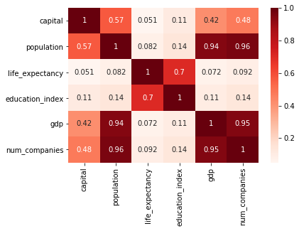
sns.heatmap(df.corr(), annot=True, cmap="Reds")
<matplotlib.axes._subplots.AxesSubplot at 0x10ba1ccf8>
Train Test Split
After some basic EDA, it's time to split the data into training and testing sets. The y (target) is going to be the population, and the rest of the columns will be the features I am using to predict the population of a city in Brazil.
y = df['population']
features = [col for col in df if col != 'population']
X = df[features]
X.head(3)
| state | capital | life_expectancy | education_index | gdp | num_companies | tourism_category | |
|---|---|---|---|---|---|---|---|
| 0 | SP | 1 | 0.855 | 0.725 | 6.870359e+08 | 530446.0 | A |
| 1 | SP | 0 | 0.840 | 0.718 | 7.440269e+07 | 15315.0 | B |
| 2 | RJ | 1 | 0.845 | 0.719 | 3.294314e+08 | 190038.0 | A |
X_train, X_test, y_train, y_test = train_test_split(X, y, test_size=0.2)
print(X_train.shape)
print(X_test.shape)
print(y_train.shape)
print(y_test.shape)
(4454, 7)
(1114, 7)
(4454,)
(1114,)
At this point in my work flow, I would import DataFrameMapper from Scikit-learn and I would start to fix each column individually. However, this is where I am going to explore a new tool to me, Scikit-Learn's ColumnTransformer, which will simultaneously transform several columns, which need the same transformation process.
Classify Columns into Categorical and Numerical
Columns do not necessarily need to be separated into these two type of columns, but in this case it makes for a better example. This is a perfect example showing when you would used DataFrameMapper and when you would use this process instead. If you have several columns that need very diferent types of transforming, I would used DataFrameMapper, if you have a more homogenous group, where you have several columns that need to be transformed in a similar way, I would use this process. It makes for a cleaner workflow.
After performing basic EDA, it became apparent that the columns State, Capital, and Tourism Category, could be defined as Categorical, and they will need to be One Hot Encoded and since there are missing values, we will need to use an Imputer. The columns Life Expectancy, Education Index, GDP, and Number of Companies, could be defined as Numerical, and they will need to be scaled, as well as have the missing values imputed.
cat_cols = ['state', 'capital', 'tourism_category']
num_cols = ['life_expectancy', 'education_index', 'gdp', 'num_companies']
Build a Pipeline for Categorical Columns
Now I am going to start building pipelines for these two types of columns. Let's start with our Categorical columns.
cat_cols #remind us what our categorical columns are
['state', 'capital', 'tourism_category']
X_train_cat = X_train[cat_cols] #pulling out the cat columns from our X_train
X_train_cat.head(3)
| state | capital | tourism_category | |
|---|---|---|---|
| 200 | SP | 0 | C |
| 3517 | SP | 0 | NaN |
| 1907 | PR | 0 | NaN |
X_train_cat.isna().sum()
state                  0
capital                0
tourism_category    1836
dtype: int64
After seeing that there are 1815 missing values, and we decide that we dont want to lose any of the valuable information in the rest of the values, we decide to impute those missing values.
si = SimpleImputer(strategy='constant', fill_value='other') #This will fill all missing values as 'other'

si.fit(X_train_cat)
X_train_cat_si = si.transform(X_train_cat)
After imputing the missing values, we will now need to one hot encode the columns.
ohe = OneHotEncoder(sparse=False)

X_train_cat_ohe = ohe.fit_transform(X_train_cat_si)
Now that we have imputed all missing values and one hot encoded the categorical columns, we will now place these two steps into a pipeline. We do this by defining them as steps and then placing them in the pipeline. The steps are an array of tuples that contain two values. The first value in a step is the name you are giving the process and the second value is the instantiated step (example si is SimpleImputer and ohe is OneHotEncoder). These steps are then placed in the pipeline and the pipe fits both the X_train and y_train.
steps = [
    ('impute', si),
    ('ohe', ohe)
]

cat_pipe = Pipeline(steps=steps)
cat_pipe.fit(X_train_cat, y_train)
Pipeline(memory=None,
     steps=[('impute', SimpleImputer(copy=True, fill_value='other', missing_values=nan,
       strategy='constant', verbose=0)), ('ohe', OneHotEncoder(categorical_features=None, categories=None,
       dtype=<class 'numpy.float64'>, handle_unknown='error',
       n_values=None, sparse=False))])
Build a Pipeline for Numerical Columns
num_cols
['life_expectancy', 'education_index', 'gdp', 'num_companies']
X_train_num = X_train[num_cols] #pulling out the numerical columns from our X_train
X_train_num.head(3)
| life_expectancy | education_index | gdp | num_companies | |
|---|---|---|---|---|
| 200 | 0.863 | 0.687 | 2530729.24 | 2464.0 |
| 3517 | 0.855 | 0.616 | 177756.32 | 213.0 |
| 1907 | 0.843 | 0.676 | 351801.06 | 731.0 |
The numerical columns need to be scaled and imputed. We could transform the columns by Standard Scaling and then transform the columns by SimpleImputing, in a two step process, like we did for the Categorical Columns, but we can actually just skip those two individual processes and place the two steps directly into the pipeline. We simply instantiate the two processes we need to complete, and then skip right to the last step, defining them within the steps and placing those steps into the pipeline.
si = SimpleImputer(strategy='mean')
ss = StandardScaler()

steps = [
    ('impute', si),
    ('ss', ss)
]

num_pipe = Pipeline(steps=steps)
num_pipe.fit(X_train_num, y_train)
Pipeline(memory=None,
     steps=[('impute', SimpleImputer(copy=True, fill_value=None, missing_values=nan, strategy='mean',
       verbose=0)), ('ss', StandardScaler(copy=True, with_mean=True, with_std=True))])
Use ColumnTransformer to Concatenate all Data Together
The ColumnTransformer can now take both pipelines, concatenating them together, to transform the entirety of the X_train.
A ColumnTransformer takes an array of tuples with three values. The first value is the name we give the process, the second value is the pipeline created, and the third value is the list of columns that the pipeline was created to transform.
transformers = [
    ('cat', cat_pipe, cat_cols),
    ('num', num_pipe, num_cols)
]

ct = ColumnTransformer(transformers=transformers)
X_train_trans = ct.fit_transform(X_train)
X_train_trans.shape
(4454, 39)
Create a Final Pipeline with a Machine Learning Model
Now we can take the transformer and a machine learning model, such as Linear Regression, and create a final pipeline that takes in all the raw data, transforms the data through the individual pipelines, concatenates the data with the transformer, and then predicts.
lr = LinearRegression()

final_steps = [
    ('transformer', ct),
    ('model', lr)
]

pipe = Pipeline(steps=final_steps)
pipe.fit(X_train, y_train)
Pipeline(memory=None,
     steps=[('transformer', ColumnTransformer(n_jobs=None, remainder='drop', sparse_threshold=0.3,
         transformer_weights=None,
         transformers=[('cat', Pipeline(memory=None,
     steps=[('impute', SimpleImputer(copy=True, fill_value='other', missing_values=nan,
       strategy='constant', ve...('model', LinearRegression(copy_X=True, fit_intercept=True, n_jobs=None,
         normalize=False))])
pipe.score(X_train, y_train)
0.9648703985990568
Now let's see if the pipeline will work on the test data. The test data was placed aside when we did our train test split. It has not been used for any of the processes above.
y_pred = pipe.predict(X_test)
y_pred
array([ 2080., 5952., 11360., ..., 5632., 30720., 15680.])
pipe.score(X_test, y_test)
0.7800829672957542
Concluding Remarks
There are many benefits to using a Scikit-learn pipeline. By enforcing and implementing the order of steps, it makes a workflow much easier to read and understand. Pipelines are especially useful, if you are working with datasets that are continuously being added to. A pipeline can be used to transform the new data in the same process.
While I am a big fan of DataFrameMapper, which can also be placed into a pipeline, I often found myself using DataFrameMapper and having to repeat myself, as many columns need the exact same transformations. With the process above, it makes it much simpler, easier, and less time consuming. While I find this new process advantageous, I need to note that there are many advantages for using DataFrameMapper. The main one that comes to mind for me is that DataFrameMapper allows you to keep the annotations and labels that you assigned to your pandas dataframe. The results of my pipeline above, on the other hand, will reduce all information to a array/matrix. This makes DataFrameMapper much easier to comprehend. Both processes have their benefits, and I envision using both in different scenarios.
Finally, pipelines can also then be used to GridSearch and find the best models and hyper-parameters. As we can see from our train and test scores, our current model is quite overfit, a GridSearch could aid in finding a model that is less overfit, and our test score could be improved.